This is a 3 part series of Deep Q-Learning, which is written such that undergrads with highschool maths should be able to understand and hit the ground running on their deep learning projects. This series is really just the literature review section of my final year report (which in on Deep Q-Learning) broken to 3 chunks:
Prologue
You can skip this. It is just me explaining how I end up publishing this.
When I was writing my final year report I was advised by my supervisor (Dr Wong Ya Ping) to write in such a way that the average layman could understand. I think he put it as “write it such that even your mom can understand” (my mom is pretty highly educated by the way). So I went out of my way to take a course on it, and kept simplifying my writing under my co-supervisor’s invaluable and meticulous review (Dr Ng Boon Yian – he is famous for reviewing final year reports). After my final year project was complete I just shelved everything and gave myself a pat in the back.
Fast forward 7 months to today. I passed my report around as reference for my juniors, and one of them commented that it was like a crash course in Convolutional Neural Networks (CNN). In a week or so, a friend from the engineering faculty was having difficulty understanding CNN, so I passed my report to him. He said it clears a lot of things up, since he had been mostly referring to the Tensorflow documentation, which is focused on teaching you how to use the library not teach you machine learning. So, with that I decided to breakdown the literature review of my report to 3 parts and publish it in my blog, in hopes to enlighten a wider audience. Hope it will clear things up for you as well!
I myself am not very focused on machine learning at the time being; I have decided to direct my attention on the study of algorithms via the Data Structures and Algorithms Specialization in Coursera. So chances are if you ask some machine learning question now I won’t be able to understand, but I’ll try. (:
Abstract
In this post, I will introduce machine learning and its three main branches. Then, I will talk about neural networks, along with the biologically-inspired CNN. In part 2, I will introduce the reader to reinforcement learning (RL), followed by the RL technique Q-Learning. In the final part, I piece together everything when explaining Deep Q-Learning.
If you are here just to understand CNN, this first part is all you need.
Types of Machine Learning
The art and science of having computer programs learn without explicitly programming it to do so is called machine learning. Machine learning, then, is about making computers modify or adapt their actions (whether these actions are making predictions, or controlling a robot) so that these actions get more accurate. Machine learning itself is divided to three broad categories (Marsland, 2015):
- Supervised Learning – We train a machine with a set of questions (inputs), paired with the correct responses (targets). The algorithm then generalizes over this training data to respond to all possible inputs. Included in this category of learning techniques is neural networks.
- Unsupervised Learning – Correct responses are not provided, but the algorithm looks for patterns in the data and attempts to cluster them together. Unsupervised learning will not be covered in this series as it is not used in Deep Q-Learning.
- Reinforcement Learning – A cross between supervised learning and unsupervised learning. The algorithm is told when the answer is wrong, but is not shown how to correct it. It has to explore different possibilities on its own until it figures out the right answer.
A system that uses these learning techniques to make predictions is called a model.
The Artificial Neural Network (ANN)
The Neuron
The simplest unit in an ANN is called a neuron. The neuron was introduced in 1943 by Warren S. McCulloch, a neuroscientist, and Walter Pitts, a logician (McCulloch & Pitts, 1943). Inspired by biological neurons in the brain, they proposed a mathematical model that extracts the bare essentials of what a neuron does: it takes a set of inputs and it either fires (1) or it does not (0). In other words, a neuron is a binary classifier; it classifies the inputs into 2 categories.

Mathematical Model of a neuron (Marsland, 2015)
In a neuron, a set of  inputs
  is multiplied by a set a weights
  (the weights are learned over time) and summed together. Both
  and
and  are typically represented as vectors.
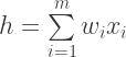
The result,  , is then passed to an activation function, which returns an output (1 or 0).
Building ANN from Neurons
A neuron by itself cannot do much; we need to put sets of neurons together into an ANN before they can be anything useful.

ANN – each circle (node) is a neuron (Karpathy et al., 2016)
What happens after we clump these neurons together to layers? How do they learn? The algorithm will learn by example (supervised learning); the dataset will have the correct output associated with each data point. It may not make sense to provide the answers, but the main goal of an ANN is to generalise over the data; finding patterns and predict new examples correctly.
To teach an ANN, we use an algorithm called back-propagation.
Back-propagation Algorithm
Back-propagation algorithm consists of two main phases, executed in order:
- Forward propagation – the inputs are passed through the ANN starting at the input layer, and predictions are made at the output layer.
- Weight update – from the predictions, we calculate how far we differ from the answer (also known as the loss). We then use this information to update the weights in the reverse direction; starting from the output layer, back to the input layer.
The weight update step is made possible by another algorithm: gradient descent.
Loss and Gradient Descent
To use gradient descent, we first need to define a loss function  , which calculates the loss. For each sample
  , loss is the difference between the predicted value
  and the actual value
  for all samples. There are various methods of calculating the loss; one of the most popular would be mean squared error function:

The goal of the ANN is then to minimize the loss. To do this we find the derivative of the loss function with respect to the weights,  . This gives us the gradient of the error. Since the purpose of learning is to minimize the loss, nudging the values of the weights in the direction of the negative gradient will reduce the loss. We therefore define the back-propagation update rule of the weights as:

 here is known as the learning rate, which is a parameter that we tweak to determine how strong we will nudge the weights with each update. An update step of the weights (including both forward and backward pass) on one sample is known as an iteration; when we iterate over all samples one time, we call this an epoch. More epochs would usually mean better accuracy, but up until the ANN converges to a possible solution. In gradient descent, 1 iteration is also 1 epoch, because the entire dataset is processed in each iteration.
Stochastic Gradient Descent
What happens if the dataset gets constantly updated with new data (transaction data, weather information, traffic updates, etc.)? There is a variation of gradient descent that allows us to stream the data piece by piece into the ANN: stochastic gradient descent (SGD). To do this a simple modification is made to the loss function (which consequently changes the derivative): instead of factoring the entire dataset in each update step we take in only a single input at a time:

For SGD, a dataset of 500 samples would take 500 iterations to complete 1 epoch. Deep Q-Learning uses SGD to perform updates to the weights (Mnih et al., 2013), using a rather unique loss function. I will elaborate on this in part 3.
Convolutional Neural Networks
Convolutional Neural Networks (CNN) are biologically-inspired variants of multi-layered neural networks. From Hubel and Wiesel’s work on visual cortex of cats (Hubel & Wiesel, 1963), we understand that the cells in the visual cortex are structured in a hierarchy: simple cells respond to specific edges, and their outputs are received by complex cells.

Hierarchical structure of the neurons (Lehar, n.d.)
In a CNN, neurons are arranged into layers, and in different layers the neurons specialize to be more sensitive to certain features. For example in the base layer the neurons react to abstract features like lines and edges, and then in higher layers neurons react to more specific features like eye, nose, handle or bottle.
A CNN is commonly composed of 3 main types of layers: Convolutional Layer, Pooling Layer, and Fully-Connected Layer. These layers are stacked together and inputs are passed forward and back according to that order.
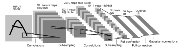
Architecture of LeNet-5, a CNN used for digits recognition (LeCun et al., 1998)
Convolutional Layer
Each convolutional layer consist of a set of learnable filters (also referred to as kernels), which is small spatially but extends through the full depth of the input volume. For example, for a coloured image (images passed into a CNN are typically resized to a square) as input, a filter on a first layer of a CNN might have size  (5 pixels width and height, and 3 color channels, RGB). During the forward pass, we slide (or convolve) each filter across the width and height of the input volume (the distance for each interval we slide is call a stride) and compute dot products between the entries of the filter and the input at any position. As we slide the filter over the width and height of the input volume we will produce a 2-dimensional activation map (also referred to as feature map). We will stack these activation maps along the depth dimension to produce the output volume (Karpathy et al., 2016), therefore the number of filters = depth of output volume.

Click image (you will need to scroll down a bit) to check out an interactive demo (built by Karpathy) of the convolutional layer at work. 2 filters, size 3*3*3, with stride of 1.
In summary, each convolutional layer requires a 3 hyperparameters to be defined: filter size (width and height only; the depth will match with the input volume), number of filters, and stride.
After an input is convolved in one layer, the output volume will pass through a Rectified Linear Units (RELU) layer. In RELU, an elementwise activation function is performed, such as:
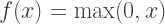
The output volume dimensions remains unchanged. RELU is simple, computationally efficient, and converges much faster than other activation functions (sigmoid, tanh) in practice.
Pooling Layer
Pooling layers performs a down sampling operation (that is why pooling operations are also called subsampling) and reduces the input dimensions. It is used to control overfitting (the state where the ANN becomes too scrupulous, and cannot generalise the input) by incrementally reducing the spatial size of the input to reduce the amount of parameters and computation in the network. Though there are many types of pooling layers, the most effective and simple is max pooling, illustrated below:
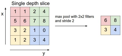
Illustration of max pooling (Karpathy et al., 2016)
There are proposed solutions to replace pooling layers altogether by simply increasing the stride (Springenberg, Dosovitskiy, Brox, & Riedmiller, 2014), and it seems likely that future architectures will either have very few to no pooling layers. Pooling layers are not used in DeepMind’s Deep Q-Learning implementation, and this will be explained later in part 3.
Fully Connected Layer
Neurons in a fully connected (FC) layer have full connections to all activations in the previous layer, as seen in regular ANN as described previously. In certain implementations such as Neon, FC layers are referred to as affine layers.
Afterword
There is a detailed writeup of CNN in the CS231n course by Karpathy: Convolutional Neural Networks (CNNs / ConvNets). I’d recommend taking a look at that for a more detailed (and more math intensive) explanation.
Of course, if you have time, the best way to get a proper foundation would be take up Andrew Ng’s machine learning course. I have gotten a cert from it, and if you are serious on this subject I’d suggest you enroll as well. Andrew even has a 5 course specialization on deep learning it now, though I won’t be taking it up anytime soon. What you will find, is that deep learning is more than just GPU’s and this magic black box called Tensorflow.
References
- Marsland, S. (2015). Machine learning: an algorithmic perspective. CRC press.
- McCulloch, W. S., & Pitts, W. (1943). A logical calculus of the ideas immanent in nervous activity. The bulletin of mathematical biophysics, 5(4), 115–133.
- Karpathy, A., Li, F., & Johnson, J. (2016). Cs231n convolutional neural network for visual recognition. Stanford University.
- Mnih, V., Kavukcuoglu, K., Silver, D., Graves, A., Antonoglou, I., Wierstra, D., & Riedmiller, M. (2013). Playing atari with deep reinforcement learning. arXiv preprint arXiv:1312.5602.
- Hubel, D., & Wiesel, T. (1963). Shape and arrangement of columns in cat’s striate cortex. The Journal of physiology, 165(3), 559.
- Lehar, S. (n.d.). Hubel & Wiesel. Retrieved 2016-08-19, from http://cns-alumni.bu.edu/~slehar/webstuff/pcave/hubel.html
- LeCun, Y., Bottou, L., Bengio, Y., & Haffner, P. (1998). Gradient-based learning applied to document recognition. Proceedings of the IEEE, 86(11), 2278–2324.
- Springenberg, J. T., Dosovitskiy, A., Brox, T., & Riedmiller, M. (2014). Striving for simplicity: The all convolutional net. arXiv preprint arXiv:1412.6806.


 pixel images) and the score (a number).
 frames, from which we then extract the luminance values. The luminance values can be calculated from RGB via the formula
  . For each input, the above preprocessing step (defined as a function
  ) is applied to 4 frames at any given time step, placing the resulting dimensions as
  .
.

 ). At a time step
  , we set a Bellman backup
  (also known as target) , followed by the loss function (de Freitas, 2014):
![L_t(w_t) = \left[y_t - Q(s, a, w_t) \right]^2](https://s0.wp.com/latex.php?latex=L_t%28w_t%29+%3D+%5Cleft%5By_t+-+Q%28s%2C+a%2C+w_t%29+%5Cright%5D%5E2&bg=ffffff&fg=333333&s=2&c=20201002)
 of the Q-function,
  , but for the target we used the previous weights
  (this is not mentioned in the research paper (Mnih et al., 2013), but it is evident in the implementation). What we are essentially doing here is approximate Bellman by minimizing the difference between current estimate reward
  and past estimate reward
  . Notice that this difference is actually the TDError as discussed earlier. So we used a supervised learning technique (neural networks), but alter the loss function that it uses a RL technique (Q-Learning). Another way to see this is to see
  :
:
 as
as  in our replay memory
  , where
  is the maximum capacity for the replay memory (a fixed constant defined by us).
 . This breaks the similarity of subsequent training samples, and makes the training task a lot more similar to supervised learning.
 -greedy policy, where
  probability exploits what it has learned.
 , we use the previous weights
  .
. , we used the previous weights
  ? We will use random weights. In implementation, this simply means we keep track of 2 weights: one of a past time step, and one of the current time step. Note that we would not necessarily need to use the weights immediately before
  , where
  is a fixed constant).
 , where
  , where
  is the set of all possible states.
 , where
  is the set of all possible actions that can be taken in the state
  .
. which returns the probability that if at time
  in the state
  we would end up in new state
  in a next time step
  .
. , which is the consequence of the action and comes 1 time step later. This value is normally an integer, and can also be negative value (punishment).
 and
and  respectively; this is useful notation in cases where time is not a consideration. Reward also has a more succinct notation:
  .
. (this is not the same as the constant pi 3.142), where
  ; a policy returns an action given a state. The best solution
  is a policy that maximizes the sum of all rewards:
 (gamma) here is called the discount rate, and is a float between 0 to 1 set by us to determine the present value of future rewards. The reward of the current state remains unchanged regardless of the discount rate (because anything to the power of 0 is 1), whereas future rewards will decay exponentially with each time step. If
  – We consider the current state, and average across all of the actions that can be taken.
 – We consider the current state and each possible action that can be taken separately. This is also known as a Q-value. A Q-state
  is when you were in a state and took an action.
 is the statistical expectation):

 (optimal state-value function); the utility starting out having taken action
  from state
  or
or 
![Q^*(s, a) = \sum_{s'} T(s, a, s') \left[ R(s, a, s') + \gamma V^*(s') \right]](https://s0.wp.com/latex.php?latex=Q%5E%2A%28s%2C+a%29+%3D+%5Csum_%7Bs%27%7D+T%28s%2C+a%2C+s%27%29+%5Cleft%5B+R%28s%2C+a%2C+s%27%29+%2B+%5Cgamma+V%5E%2A%28s%27%29+%5Cright%5D&bg=ffffff&fg=333333&s=2&c=20201002)
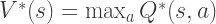
![V^*(s) = \max_a \sum_{s'} T(s, a, s') \left[ R(s, a, s') + \gamma V^*(s') \right]](https://s0.wp.com/latex.php?latex=V%5E%2A%28s%29+%3D+%5Cmax_a+%5Csum_%7Bs%27%7D+T%28s%2C+a%2C+s%27%29+%5Cleft%5B+R%28s%2C+a%2C+s%27%29+%2B+%5Cgamma+V%5E%2A%28s%27%29+%5Cright%5D&bg=ffffff&fg=333333&s=2&c=20201002)
 ) is the reward of the current state multiplied by future expected rewards of the consequent state; this is recursively denoted as
  . To prioritize the reward of the current state we apply a discount rate
  are, the next step is to compute the these optimal utilities. To do this we use the value iteration algorithm.

 . The estimated utility then becomes:

 is also called TDError or temporal difference error.
 ![Q(s, a) \gets Q(s, a) + \alpha \left[y - Q(s, a)\right]](https://s0.wp.com/latex.php?latex=Q%28s%2C+a%29+%5Cgets+Q%28s%2C+a%29+%2B+%5Calpha+%5Cleft%5By+-+Q%28s%2C+a%29%5Cright%5D&bg=ffffff&fg=333333&s=2&c=20201002)

 , but instead choose the one that gives the highest value. This is known as an off-policy decision.


 (read as omega):
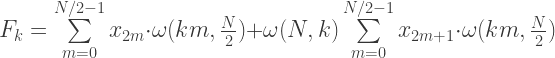

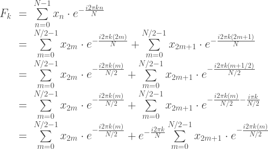
 you only need to compute
  a total of
  times; we can essentially half the number of computations using this technique. But why stop there? We can also take either
  or
or  and split them to odd and even parts, and repeat the same procedure. If we compute this recursively, the base case for this is when
  . In this manner we compute
  . Therefore, for sequence of size N, FFT computes the DFT in
  time.
time.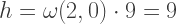


 .
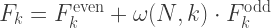
.

 , though not visually depicted. The whole computation flow shows a sort of “butterfly pattern”, as how most engineers like to describe it.
 .
. . In FFT we resize N to the closest power of 2, which is 256.
 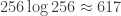 . That is 2697% less computations! Of course, it shouldn’t be hard to convince yourself that this is still true as N gets larger.
 ), the index 7 (0111) with be swapped with 14 (1110).