1-0 Knapsack Problem – A Hands-on Guide (C++)

Posted on December 14, 2015 by Lee Zhen Yong

The 1-0 knapsack problem; an optimization puzzle famously solved with dynamic programming (dp). This post is merely my take on the problem, which I hope to provide a more hands-on approach.

To get started, try and attempt The Knapsack Problem (KNAPSACK) from SPOJ. Study the problem closely as I will referring to it throughout this guide. I will then explain how the general solution is derived and how dp is applied.

I assume you have known a bit of dp as a prerequisite, though if you haven’t you can check out my beginner friendly hands-on intro: 445A – Boredom – CodeForces Tutorial.

The General Solution

A dp solution is usually derived from a recursive solution. So let’s start with that.

We define 2 containers: v and c, that contains the all the values of each item and the capacity they consume respectively, starting from index 1. So for example, v[2] and c[2] returns the value and size of the 2nd item.

What are we trying to optimize here? We are trying to maximize the value; the combination of items that yields the highest value. So let us define a function B(i, w) that returns the maximum value given a scope of items (i) and the capacity of the knapsack (w). The solution to KNAPSACK will therefore be B(N, S).

In solving it recursively, imagine we have all N items with us and our knapsack completely empty (current capacity is S), and we consider the items one by one from the last one (the N-th item).

What are the base cases of this problem? When there are no items to put in (i = 0), or when the knapsack cannot contain any items (w = 0).

Before we consider some i-th item, we first need to make sure that it can fit into the knapsack given its capacity, in other words, an i-th item should not be considered if c[i] > w. If this is so, you will consider the maximum value of the the scope of items excluding the i-th item, or B(i-1, w).

So what happens when you can put the item in the knapsack? You have 2 choices: To put it in (take), or not put it in (keep).

Keep: you exclude it from the scope of items in which you consider the maximum value, which is again B(i-1, w).
Take: you will get the value of the i-th item you select (v[i]), BUT, we should also consider the remaining space after adding the i-th item inside (w-c[i]). When considering items to add here, we need to exclude the item we already added, so the scope of items we consider is i-1. With this remaining space and this scope of items, we also want to get the maximum value. We can do this recursively via B(i-1, w-c[i]).

Choosing between keep and take is as simple as taking the maximum of the 2.

If you piece all this together, you will get the general solution:

$B(i,j) = \begin{cases} 0 \text{ if } i = 0\text{ or }w = 0\\ B(i-1, w) \text{ if } c[i] > w\\ max\Big( B(i-1, w), v[i] + B(i-1, w-c[i]) \Big) \end{cases}$

Recursive Solution

Short and simple:

	#include <iostream>
	#include <vector>
	#include <algorithm>

	using namespace std;

	vector<int> v, c;

	int B(int i, int w)
	{
	if (i == 0 \|\| w == 0) return 0;
	if (c[i] > w) return B(i – 1, w);

	return max(B(i – 1, w), v[i] + B(i – 1, w – c[i]));
	}

	int main()
	{
	int S, N; cin >> S >> N;

	// sloted in for easy array access; values won't be used.
	c.push_back(-1);
	v.push_back(-1);

	int ct, vt;
	for (int i = 0; i < N; i++) {
	cin >> ct >> vt;
	c.push_back(ct);
	v.push_back(vt);
	}

	cout << B(N, S);
	}

view raw

knapsack-recursive.cpp

hosted with ❤ by GitHub

Plug it in the judge and you will get a TLE (Time Limit Exceeded).

Dynamic Programming Solution

We use a 2D array, DP, containing N+1 rows and S+1 columns. The rows map to the scope of i items we consider (the top considers 0 items and the bottom considers all N items). The columns map to capacity (an individual column is denoted as the w-th column) of knapsack left to right from 0 to S. A cell DP[i][w] means “this is the maximum value given i items and capacity of w“. The maximum value for N items and capacity of S is therefore DP[N][S].

We first fill DP with base cases: where i = 0 and where w = 0. This means that the first row and first column are all 0. The order in which we solve this is simple: starting where i = 1 and w = 1, for each row from top to bottom, we fill the cells from left to right.

I will continue on with an example using inputs from Tushar Roy’s YouTube video (you should check it out), but I jumbled the order to prove that ordering of items is not important. Here is the DP array:

Cells shaded in pale blue is when item does not fit in capacity w, or where c[i] > w. In pale green cells we have a choice: keep or take. Notice that with every row, we are adding one more item to consideration, and with every column we increase the capacity by 1.

Here is the code:

	#include <iostream>
	#include <vector>
	#include <algorithm>

	using namespace std;

	int main()
	{
	vector<int> v, c;
	int S, N; cin >> S >> N;

	// sloted for easy array access; values won't be used.
	c.push_back(-1);
	v.push_back(-1);

	int ct, vt;
	for (int i = 0; i < N; i++) {
	cin >> ct >> vt;
	c.push_back(ct);
	v.push_back(vt);
	}

	vector< vector<int> > DP(N + 1, vector<int>(S + 1, 0));

	for (int i = 1; i <= N; i++) { // i is scope of items in consideration
	for (int w = 1; w <= S; w++) { // j is max size of bag
	if (c[i] > w) {
	DP[i][w] = DP[i – 1][w];
	} else {
	DP[i][w] = max(DP[i – 1][w], v[i] + DP[i – 1][w – c[i]]);
	}
	}
	}

	cout << DP[N][S];
	}

view raw

knapsack-dp.cpp

hosted with ❤ by GitHub

Getting the Selected Items

Some people use an auxiliary Boolean array (often called Keep) that keeps track of whether an item is selected or not. This seems to be an unnecessary occupation of space to me, since you can deduce the selected items from DP itself.

You start from DP[N][S], and from there:

An item is selected, if the value of the cell directly above it is not equal to the current cell. When this happens, the capacity of the knapsack reduces by the weight of the selected item. With that new capacity you select the next item.
An item is not selected, if the value of the cell directly above it is equal to the current cell. So we consider the next item by moving up one row; capacity remains unchanged.

This process continues until either there are no more items remaining, or the knapsack is full.

The table below shows the trail of the algorithm as it selects items (item 1 and 4) from the DP array we constructed before:

Below is the recursive function:

void pick(int i, int w)
{
    if (i <= 0 || w <= 0) return;

    int k = DP[i][w];
    if (k != DP[i - 1][w]) {
        cout << i << " "; // select!
        pick(i - 1, w - c[i]); // capacity decreases
    } else {
        // move on to next item; capacity no change
        pick(i - 1, w);
    }
}

See the full implementation of this function in this gist.

Application

Enough spoon feeding! It is time for you to try out some puzzles on your own. Conveniently UVa grouped a series of 3 questions that are slight variations of the 1-0 knapsack problem. I sort them here in order of difficulty:

10130 – SuperSale (my solution)
990 – Diving for Gold (my solution)
– You will need to list down the items you select in this one.
– Beware of the tricky formatting! There shouldn’t be a blank line at the end of your output.
562 – Dividing coins (my solution)
– In my solution, there is a tip (short comment block before the main function) you can check out if you just want some pointers to get started.

References

Dynamic Programming | Set 10 ( 0-1 Knapsack Problem) (www.geeksforgeeks.org/)
Dynamic-Programming Solution to the 0-1 Knapsack Problem (www.personal.kent.edu)

Matrix Chain Multiplication with C++ code – PART 3: Extracting the Sequence

Posted on November 24, 2015 by Lee Zhen Yong

In my previous post, I wrote about finding the minimum cost of multiplying a matrix chain using dynamic programming. In this post I build on top of what we have covered to extract the sequence of multiplying the chain itself.

This is part of a 3 part series:

Analysis and Design – analyze the problem and deduce a solution.
Implementation – implement the algorithm to find the minimum number of operations.
Extracting the Sequence – extract the sequence in which the chain is multiplied.

Extract the Sequence

To do this we keep track of the point at which we split up the chain as prefix and suffix: the point k (we define this from the previous post). We do this by storing it in another 2D array of the same size as DP, which we call splits:

int ops = DP[i][k] + DP[k + 1][j] + rc[i] * rc[k + 1] * rc[j + 1];
if (ops < DP[i][j]) {
	DP[i][j] = ops;
	splits[i][j] = k;
}

Now let us print out the elements of splits in dark blue. I will be reusing the example input from the previous post:

How do we interpret this? Let us start from where we got the main solution; where i = 1 and j = 6. This cell splits[1][6] signifies the last operation of multiplying the matrix chain – in the above table this maps to 3. This means in the last operation, a prefix from a chain $A_1 \ldots A_3$ multiplies with a suffix from a chain $A_{4} \ldots A_6$ .

Let us now consider just the prefix. How then is prefix $A_1 \ldots A_3$ multiplied? We find that from splits[1][3], which in this case is 1. Therefore the it is formed by multiplying a prefix $A_1 \ldots A_1$ and a suffix $A_2 \ldots A_3$ . In this prefix $A_1 \ldots A_1$ we hit a base case where i = j. Should this happen we return the matrix $A_1$ . The suffix $A_2 \ldots A_3$ is split from from splits[2][3], which is 2. This in turns hits 2 base cases and returns the matrix $A_2$ and $A_3$ .

If you repeat this recursive process with the top level suffix, you parenthesize the chain as such:

We can generalize a function mult that returns the resultant matrix that has been multiplied in the most optimal way from the matrix chain:

$mult(i, j)=\begin{cases}A_i \text{ if } i = j\\mult(i, k) \cdot mult(k+1, j)\text{ where } k = splits[i][j]\end{cases}$

The main solution is therefore mult(1, 6).

Implementation

Below is an implementation of this:

	#include <algorithm>
	#include <iostream>
	#include <vector>
	#include <climits>
	#include <string>

	using namespace std;

	vector<int> rc;
	vector< vector<int> > DP, splits;

	string mult(int i, int j)
	{
	if (i == j) {
	return to_string(i); // Basis
	} else {
	int k = splits[i][j];
	string X = mult(i, k);
	string Y = mult(k + 1, j);
	cout << "multiply " << X << " and " << Y << endl;
	return "(" + X + "*" + Y + ")";
	}
	}

	int main()
	{
	int c; cin >> c;
	int n = c – 1;
	rc = vector<int>(c + 1, -1);
	DP = splits = vector< vector<int> >(c, vector<int>(c, 0));
	int x;

	// for every matrix i, rc[i] is row and rc[i+1] is column
	for (int i = 1; i <= c; i++) {
	cin >> x;
	rc[i] = x;
	}

	for (int w = n; w > 0; w–) {
	int p = n – w;
	for (int j = n; j > p; j–) {
	int i = j – p – 1;
	DP[i][j] = INT_MAX;
	for (int k = i; k < j; k++) {
	int ops = DP[i][k] + DP[k + 1][j] + rc[i] * rc[k + 1] * rc[j + 1];
	if (ops < DP[i][j]) {
	DP[i][j] = ops;
	splits[i][j] = k;
	}
	}
	}
	}

	cout << mult(1, n);
	}

view raw

mat-chain-mult-dp-trace.cpp

hosted with ❤ by GitHub

Because we don’t have the contents of the matrices, I have the program output the parenthesis instead, along with the order in which it parenthesize them:

./mat-chain-mult-dp-trace < input.txt
multiply 2 and 3
multiply 1 and (2*3)
multiply 4 and 5
multiply (4*5) and 6
multiply (1*(2*3)) and ((4*5)*6)
((1*(2*3))*((4*5)*6))

Note that the numbers here are not integers but indices that map to its respective matrix in the matrix chain.

It is not that hard to convert the above code to multiply matrices. I will leave it as an exercise, should you be interested.

Application

Why is this matrix chain multiplication problem so important that most computer science undergraduate programs must include it in their syllabus? The same reason applies for most algorithms you learn: some problems are just slight variations of another problem. Understanding one solution to a problem in the marrow of its bones may help you solve another similar problem.

Therefore, I encourage you to challenge yourself on these 2 problems to help solidify your understanding:

You can find my solutions to these problems in my github SPOJ repository.

Reference

Algorithms – Lecture 10: Dynamic Programming, Matrix Chain Multiplication and Typesetting (video lecture by Abhi Shelat of the University of Virginia)
Matrix-chain Multiplication Problem (www.personal.kent.edu/)

Matrix Chain Multiplication with C++ code – PART 2: Implementation

Posted on November 19, 2015 by Lee Zhen Yong

In the last post I explained how we got the general solution:

$B(i,j) = \begin{cases} 0 \text{ if } i = j \\ \displaystyle\min_{k=i}^{j-1} \begin{cases} B(i, k) + B(k+1, j) + r_i \cdot c_k \cdot c_j \end{cases} \end{cases}$

In this post we plug the formula in and watch it run! I will go through the recursive solution ( $O(2^n)$ ), and then the more optimal dynamic programming solution ( $O(n^3)$ ).

This is part of a 3 part series:

Analysis and Design – analyze the problem and deduce a solution.
Implementation – implement the algorithm to find the minimum number of operations.
Extracting the Sequence – extract the sequence in which the chain is multiplied.

Input

Our input (input.txt), therefore, is the rows and columns of all n matrices:

7
30 35 15 5 10 20 25

The above input meant that there are 7 integers that correspond to the dimensions of 6 matrices:

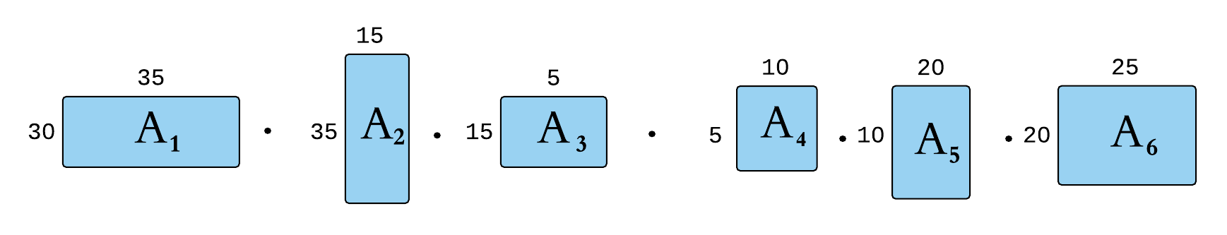
The input only contains the rows from matrix $A_1$ until $A_6$ , followed by the column of matrix $A_6$ . This is because a matrix A and only be multiplied with a matrix B if they are compatible (if $r_A = c_B$ ). So for brevity sake we do not need to put rows and columns of all matrices (otherwise the sequence will look like 30 35 35 15 15 5 5 10 10 20 20 25).

Notice, that if we place the sequence of integers in an array rc, the row of a matrix $A_i$ is rc[i] and the column is rc[i+1].

Recursive Implementation

As surprising though it may be, the amount of code is surprisingly little:

	#include <iostream>
	#include <vector>
	#include <climits>
	#include <algorithm>

	using namespace std;

	vector<int> rc;

	int B(int i, int j)
	{
	if (i == j) return 0;

	int mink = INT_MAX;
	for (int k = i; k < j; k++) {
	mink = min(mink, B(i, k) + B(k+1, j) + rc[i]rc[k+1]rc[j+1]);
	}

	return mink;
	}

	int main()
	{
	int c; cin >> c;
	rc = vector<int>(c+1, -1);
	int x;

	// for every matrix i, rc[i] is row and rc[i+1] is column.
	for (int i = 1; i <= c; i++) {
	cin >> x;
	rc[i] = x;
	}

	int n = c – 1;
	cout << B(1, n);
	}

view raw

mat-chain-mult-recursive.cpp

hosted with ❤ by GitHub

I have written the code to follow the formula as close as possible, as such I start the index with 1 instead of 0. You can always change it to save that bit of space, but the code just serves to show that it works:

./mat-chain-mult-recursive < input.txt
15125

Now, if you print the inputs of the function B each time it is being called, you will see a lot of the same inputs are being called again and again. In geeksforgeeks.org’s article on matrix chain multiplication, they took the time to draw out the recursion tree.

Dynamic Programming: Ordering

So now we have broken the main problem to small recurring subproblems (Overlapping Subproblems), which we can piece together to solve the main problem (Optimal Substructure). With this 2 properties, we can use dynamic programming to drastically reduce the running time of an exponential solution.

However, this problem is tricky to solve since it involves 2 variables i and j. We need a 2D array to keep track of this. In a single dimensional array ordering is trivial; we simply go from left to right, building the solution from the bottom up, but with 2 dimensions ordering becomes tricky. Which cell do we solve first?

Well, we know that:

the base case is when i = j, then B(i, j) = 0.
i cannot exceed j, so those areas will need to be grayed out.
B(1, 6) is the solution.

So with that, let us fill up an array DP based on the inputs we have above:

So we need to find B(1, 6) yes? Well, what does B(1, 6) need? Well, if we unfold the general solution plugging in i as 1 and j as 6 we have 5 selections in which we choose the smallest:

$\begin{cases}k=1: B(1, 1) + B(2, 6) + r_1 \cdot c_1 \cdot c_6 \\k=2: B(1, 2) + B(3, 6) + r_1 \cdot c_2 \cdot c_6 \\k=3: B(1, 3) + B(4, 6) + r_1 \cdot c_3 \cdot c_6 \\k=4: B(1, 4) + B(5, 6) + r_1 \cdot c_4 \cdot c_6 \\k=5: B(1, 5) + B(6, 6) + r_1 \cdot c_5 \cdot c_6 \end{cases}$

To make it easier to visualize what B(1, 6) requires, I distinguish the selection by colour:

What you can see, is that B(1, 6) requires cells to the left and to the bottom of it. Well, we have the cells that represent the base cases solved. Perhaps the next logical step is to solve the next diagonal. This is possible, because all the values of all cells where j – i = 1 depends on all cells where j – i = 0. Consequently, all values of all cells where j – i = 2 depends on all cells where j – i = 1 and j – i = 0; you can validate this by plugging in the numbers into the formula. Because all cells aside the base case requires cells below and to its left up until it hits the base case, we can continue filling up the cells of the array DP diagonally until we hit the top right cell.

From another perspective, we are finding all 5 pairs of the matrices in the chain and find their minimum cost (choose from 1 each), then we find all 4 triplets of matrices in the chain and find their minimum cost (choose from 2), then we find all 3 quadruplets of matrices in the chain and find their minimum cost (choose from 3), and this repeats until we hit the top right cell; each subsequent pass depending on the pass before it.

So we solve in diagonals in order j – i = 0, 1, 2 … n – 1. Once you can sequentially iterate through the array DP in a diagonal fashion, you have everything you need to piece together the solution:

It helps that you calculate the cells by hand to grasp the essence of this algorithm.

Dynamic Programming: Implementation

So what I did, was design a nested for loop to print the indices in the order I want. Once I do that I simply plug the formula inside, and I have my final solution:

	#include <algorithm>
	#include <iostream>
	#include <vector>
	#include <climits>

	using namespace std;

	vector<int> rc;
	vector< vector<int> > DP;

	int main()
	{
	int c; cin >> c;
	int n = c – 1;
	rc = vector<int>(c+1, -1);
	DP = vector< vector<int> >(c, vector<int>(c, 0));
	int x;

	// for every matrix i, rc[i] is row and rc[i+1] is column
	for (int i = 1; i <= c; i++) {
	cin >> x;
	rc[i] = x;
	}

	for (int w = n; w > 0; w–) {
	int p = n – w;
	for (int j = n; j > p; j–) {
	int i = j – p – 1;
	DP[i][j] = INT_MAX;
	for (int k = i; k < j; k++) {
	DP[i][j] = min(DP[i][j], DP[i][k] + DP[k + 1][j]
	+ rc[i] * rc[k + 1] * rc[j + 1]);
	}
	}
	}

	cout << DP[1][n];
	}

view raw

mat-chain-mult-dp.cpp

hosted with ❤ by GitHub

Note that again, the index starts at 1.

Although code count is near indistinguishable, the performance is drastically improved at a negligible expense of space. We generalize that the improved implementation is $O(n^3)$ by counting the number of nested for loops.

Conclusion

In the 3rd and final part, I will guide you through extracting the actual order in which the chain is multiplied. Check it out: Matrix Chain Multiplication with C++ code – PART 3: Extracting the Sequence.

References

Algorithms – Lecture 10: Dynamic Programming, Matrix Chain Multiplication and Typesetting (video lecture by Abhi Shelat of the University of Virginia)
Dynamic Programming | Set 8 (Matrix Chain Multiplication) (www.geeksforgeeks.org)

Matrix Chain Multiplication with C++ Code – PART 1: Analysis and Design

Posted on November 15, 2015 by Lee Zhen Yong

Ah. The matrix chain multiplication problem. A classic dynamic programming example in the undergraduate computer science world. I will be doing a series consisting of 3 parts:

Analysis and Design – analyze the problem and deduce a solution.
Implementation – implement the algorithm to find the minimum number of operations.
Extracting the Sequence – extract the sequence in which the chain is multiplied.

There’s practically a ton of articles out there that already writes about this problem. I intend to distinguish myself by expressing it in the simplest terms possible with examples, and season it with working C++11 source code. In other words, if you had problem understanding everywhere else, my hopes is that your search ends with this series.

In this first part, there will be no code. At all. Not even pseudocode. I promise some C++11 code in the coming 2 parts, but understanding this section will be important for implementation later.

Prerequisites

I will assume you should have a bit of background in matrix math. It helps that you do a bit of refreshing if you have forgotten.

I will also assume you have known a bit of what dynamic programming is, as matrix chain multiplication is a slightly more complex example; you keep track of a 2D array instead of 1D array. I’ve written a beginner level hands on introduction to dynamic programming in a form of solving a problem which you can check out: 445A – Boredom – CodeForces Tutorial.

Understanding the Problem

Given a chain of matrices, we want to multiply them. We cannot change the order of the matrices as that would change the result or make it incompatible, therefore we say matrix multiplication is not commutative. In addition, regardless of how you parenthesize (e.g. whether the sequence as multiplied as $A\cdot \left ( B\cdot C \right )$ or $\left ( A\cdot B \right )\cdot C$ ) the chain it will give you the same answer, thus we say it is associative.

How we parenthesize the matrices also determine how many operations will be performed. For a multiplication chain of integers, parenthesizing them does not affect the number of operations performed, but for matrices the change is significant. For example, given the matrices with the following dimensions:

If we define a row of a matrix as $r_A$ and the column as $c_A$ , then the total number of multiplications required to multiply A and B is $r_A \cdot c_A \cdot c_{B}$ .

$A\cdot \left ( B\cdot C \right )$ -> 2*20*1 + 2*1*10 = 60 multiplications
$\left ( A\cdot B \right )\cdot C$ -> 20*1*10 + 2*20*10 = 600 multiplications

The 1st case is 10 times faster!

NOTE: There is a neat coding exercise you can try out on this total multiplications thing on UVa.

Therefore, we want to figure out how to parenthesize the matrix chain such that we minimize the required number of operations.

However, to keep things simple, we will focus on the minimum number of operations. We will eventually find the sequence itself by building on top on this.

Formulation

To put in formal terms, given a sequence of n matrices $A_1, A_2, A_3 \ldots A_n$ we wish to parenthesize the product of this sequence so as to minimize the number of operations required.

Finding the Minimum Number of Operations

Suppose we have a function B(i, j) that computes the minimum number of required operations for multiplying a chain of matrices from matrix i to matrix j. The solution to the main problem would be B(1, n).

A standard technique to in solving a dynamic programming problem is usually to ask, “What is the last operation?”. Here, we ask what is the minimum total cost of the last operation? Regardless how the chain is parenthesized, there will always be 2 matrices remaining. The cost, is the minimum cost of some prefix + minimum cost of some suffix + the number of operations to multiply them. The cost of prefix and suffix in turn, is derived from the minimum number of operations that deduces them.

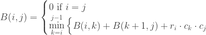
Because each matrix can only multiply with its adjacent matrix, a prefix can only start from $A_1$ to some matrix $A_k$ , and a suffix can only start from $A_{k+1}$ to $A_n$ , split at some index k. The cost in the last operation for the prefix is then B(1, k) and the cost of the suffix is B(k+1, n). k therefore ranges from 1 until n-1 in the last operation, and within a range i to j, k ranges from i to j-1. We choose k by selecting the minimum cost of all the possible costs within a range i to j.

The resultant dimensions from multiplying 2 matrices are important to finding the cost. In a sequence of matrices $A_i \ldots A_j$ If we split at a point k, the resultant dimensions of the prefix is $r_i \times c_k$ and the suffix is $r_{k+1} \times c_j$ . The cost of multiplying these 2 matrices are therefore $r_i \cdot c_k \cdot c_j$ .

Running Through Possibilities

Let us consider the base case: When there is only 1 matrix. The prefix = suffix, and there are no operations performed, so the cost = 0.

Now what if there are only 2 matrices? There are no other possible combinations to compare with, so the minimum number of operations is the number of operations to multiply them. There is no cost to the prefix or suffix, because the cost for 1 matrix alone is 0.

3 matrices onwards is gets a little more challenging. When the chain has only 3 matrices, you have to choose between $\left ( A_1\cdot A_2 \right )\cdot A_3$ and $A_1\cdot \left ( A_2\cdot A_3\right )$ . How we choose between the 2 is determined by cost of either multiplying $A_1$ and $A_2$ first, then take the resulting matrix (prefix) and multiply by $A_3$ (suffix), OR, multiplying $A_2$ and $A_3$ first, then multiplying that (suffix) by $A_1$ (prefix). Where we decide to make that split, either at $A_1$ or $A_2$ , we determined by their cost. The matrix in which we choose we call it $A_k$ , at a point k.

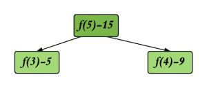
The minimum cost with 3 matrices, B(1, 3) is therefore $B(1, k) + B(k+1, 3) + r_1 \cdot c_k \cdot c_3$ , and we choose between $B(1, 1) + B(2, 3) + r_1 \cdot c_1 \cdot c_3$ and $B(1, 2) + B(3, 3) + r_1 \cdot c_2 \cdot c_3$ . You can continue doing this for 4 or 5 or 6 matrices until you start to see a pattern. Notice you can apply the same procedure to find B(1, 3) to find B(1, 2) – there is only 1 possible value for k for B(1, 2).

The General Solution

So in a range i to j, we select from j – i possibilities, from i until j – 1. Those possibilities in turn call B recursively until it hits the base case where i = j. The general solution is therefore:

$B(i,j) = \begin{cases} 0 \text{ if } i = j \\ \displaystyle\min_{k=i}^{j-1} \begin{cases} B(i, k) + B(k+1, j) + r_i \cdot c_k \cdot c_j \end{cases} \end{cases}$

And the solution to the main problem would be B(1, n).

Conclusion

This is all for the first part. Next post I will cover implementation: Matrix Chain Multiplication with C++ code – PART 2: Implementation.

Reference

Algorithms – Lecture 10: Dynamic Programming, Matrix Chain Multiplication and Typesetting (video lecture by Abhi Shelat of the University of Virginia)
Matrix-chain Multiplication Problem (www.personal.kent.edu/)

445A – Boredom – CodeForces Tutorial

Posted on November 8, 2015 by Lee Zhen Yong

Inasmuch as this is a CodeForces tutorial, I’d also want to use Boredom as an introduction to dynamic programming (dp). I will also compare the dp solution to its alternate recursive implementation. This tutorial also caters to people who can’t seem to wrap their head around the solution or tutorial from CodeForces.

I won’t be explaining the problem itself. Should be pretty straightforward.

Gotchas

The maximum points can exceed the limit for the 32-bit data type int. In some of the test cases that value can be as high as 9999899998 (the maximum capacity for 32-bit int is 2147483647). The maximum value for the n integers may be up to 10^5, but they can total up to a lot higher than that.

That is why you will see C/C++ solutions out there the data type long long int:

typedef long long int bigInt;

Solution Overview
You can try to understand the succinct tutorial from CodeForces, if you haven’t already looked into it.
The sequence of n numbers needed to be grouped together and kept count, because when selecting a single number, it makes sense to repeatedly select it (thereby adding it to your points) until it doesn’t exist in the sequence. We will keep track of this count in array c, where c[i] contains the number of occurrences of i.
Let f be a function that calculates the maximum number of points to a value up to i. Now there will be 2 base cases:

If i = 0, then f(0) = 0
If i = 1, then f(1) = c[1]

I hope the 2nd point is clear. Up to 1 the maximum number of points you can get by selecting 1 is the number of occurrences of 1 in the array c.
When i >= 2, you have 2 choices in deciding which will be f(i):

Select f(i – 2), in which you can also add with i * c[i].
Select f(i – 1), but in doing so you can’t choose to add i * c[i] because of the condition that all elements equal to a_k + 1 and a_k - 1 also must be deleted from the sequence.

Choosing between 1 and 2 is as simple as choosing which is largest.
Now let m be the largest number in the sequence. The solution is therefore f(m). The CodeForces tutorial writes f(n), but n here implies the number of elements in the sequence. To avoid confusion, I used m instead.
Most implementations I see online simply put f(100000).
It helps that you trace the algorithm step by step on paper, should it not be apparent to you how it works. For example for input:
10
10 5 8 9 5 6 8 7 2 8
You can track the values of i, c[i], and f(i):
i    c[i]   i*c[i]   f(i)
0    0      0        0
1    0      0        0
2    1      2        2
3    0      0        2
4    0      0        2
5    2      10       12
6    1      6        12
7    1      7        19
8    3      24       36
9    1      9        36
10   1      10       46
Do not undermine this method; learning how to trace algorithms in a systematic way can be very helpful to help you understand it.
Recursive Implementation
Based on the solution as detailed above, here the recursive implementation.
#include &lt;algorithm&gt;
#include &lt;iostream&gt;
#include &lt;vector&gt;

typedef long long int bigInt;

using namespace std;

vector&lt;bigInt&gt;  c(100001, 0);

bigInt f(const int i)
{
    if (i == 0) return 0;
    if (i == 1) return c[1];

    return max(f(i - 1), f(i - 2) + i*c[i]);
}

int main()
{
    int n, x, m = 0;
    cin &gt;&gt; n;

    while(n--) {
        cin &gt;&gt; x;
		c[x]++;
		m = max(m, x);
	}

	cout &lt;&lt; f(m);
}

Don’t submit this solution; it will fail at test 9 (time limit exceeded).
That’s it! In 30 lines of code you can solve this problem! The issue? Well, try and increase the values in the sequence (not the number of elements in the sequence. This doesn’t affect the growth of the function). Even a value as small as 30 and I had to wait a few seconds for it to compute.
Analysis of Recursive Implementation
We can define the performance of this recursive implementation by the number of recursive calls.
Let us trace the recursive calls of the function f in a recursion tree. I used paler colors to signify the depth of the recursion tree; the deeper it gets, the paler it gets:

That is a total of 9 recursive calls. How about f(5)?

5+9+1 (including itself) = 15 function calls.
If you observe for awhile, you will be able to deduce a pattern. Let q be a function that finds the number of function calls for f given i. Then we write q as: q(i)=q(i-1) + q(i-2) + 1, for all i >= 2; q(0)=1; q(1)=1. If you plot this function as a graph, you will get this:

So time complexity is O(2^n); Implementation scales exponentially.
By the time i reaches 18, q(18) = 8361. When i = 30, the number of function calls becomes 2692537! This would explain that bit of lag earlier. Just imagine i going as big as 10000. It is no surprise then, that when this happens, the program crashes due to stack overflow:

Dynamic Programming Implementation
Dynamic programming, in essence, is an optimization technique that dramatically cuts down computational time but taking out a bit of space to store calculated answers to overlapping subproblems. The overlapping subproblems here are the calls to f, which for example in the recursion tree f(4) we can see that f(1) is called 3 times and f(2) and f(0) is called 2 times.
Furthermore, we can take the solutions the subproblems to compute the solution of the main problem. For example f(5) can be determined by f(4) and f(3), and f(4) can be determined by f(3) and f(2), and so on. This property is called Optimal Substructure.
To recap, the 2 properties that must exist for a problem to be made solvable by dp:

Overlapping Subproblems
Optimal Substructure

Let’s put theory to practice.
We can reduce the time complexity from O(2^n) to O(n) by keeping an array DP of the same size as c. DP will store the calculated values of f for all i. The solution, therefore, is DP[m], since it contains f(m). Below is the dynamic programming solution:
#include &lt;algorithm&gt;
#include &lt;iostream&gt;
#include &lt;vector&gt;

typedef long long int bigInt;

using namespace std;

int main()
{
	const int MAX_N = 100001;

	int n, x;
	vector&lt;bigInt&gt; dp(MAX_N, 0);
	vector&lt;bigInt&gt;  c(MAX_N, 0);

	cin &gt;&gt; n;

	while(n--) {
		cin &gt;&gt; x;
		c[x]++;
	}

	dp[0] = 0;
	dp[1] = c[1];

	for (int i = 2; i &lt; MAX_N; i++) {
		dp[i] = max(dp[i - 1], dp[i - 2] + i*c[i]);
	}

	cout &lt;&lt; dp[MAX_N - 1];
}

In the dp solution, f(i) is computed from 0 to 10000 (bottom to top), whereas in the recursive solution f(i) is computed from m to 0 (top to bottom).
Notice I didn’t bother keep track the largest value in the sequence (variable m). You can have that bit of optimization if you use it, but it isn’t necessary for this problem. In essence we have f (the block of code inside that for loop) called a constant 10000 times each time this program is called, and this works granted the largest value in the sequence doesn’t exceed 10000.
What is fascinating about this implementation is that it solves the problem with the same amount of code! Ladies and gentlemen, the power of algorithms!
References

CS 383, Algorithms Dynamic Programming (www.cs.bc.edu)
What is the algorithmic approach to solve the Codeforces problem “Boredom”? (Quora.com)
Codeforces #260(Div 1) A.Boredom (codinghangover.wordpress.com)

Bruceoutdoors Blog of Blots

Yet another blog of technical ramblings!

Tag Archives: dynamic programming

1-0 Knapsack Problem – A Hands-on Guide (C++)

The General Solution

Recursive Solution

Dynamic Programming Solution

Getting the Selected Items

Application

References

Matrix Chain Multiplication with C++ code – PART 3: Extracting the Sequence

Extract the Sequence

Implementation

Application

Reference

Matrix Chain Multiplication with C++ code – PART 2: Implementation

Input

Recursive Implementation

Dynamic Programming: Ordering

Dynamic Programming: Implementation

Conclusion

References

Matrix Chain Multiplication with C++ Code – PART 1: Analysis and Design

Prerequisites

Understanding the Problem

Formulation

Finding the Minimum Number of Operations

Running Through Possibilities

The General Solution

Conclusion

Reference

445A – Boredom – CodeForces Tutorial

Gotchas

Solution Overview

Recursive Implementation

Analysis of Recursive Implementation

Dynamic Programming Implementation

References