Deep Q-Learning 101: Part 3 – Deep Q-Learning

This is a 3 part series of Deep Q-Learning, which is written such that undergrads with highschool maths should be able to understand and hit the ground running on their deep learning projects. This series is really just the literature review section of my final year report (which in on Deep Q-Learning) broken to 3 chunks:

• Part 1 – Convolutional Neural Networks
• Part 2 – Reinforcement Learning
• Part 3 – Deep Q-Learning

Introduction: The Atari 2600 Challenge

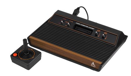
The Atari 2600 (or Atari VCS before 1982) is a home video game console released on September 11, 1977 by Atari, Inc.

Atari 2600 with standard joystick

The challenge is as follows: can an AI, given the same inputs as human player, play a variety of games without supervision? In other words, if the AI can hold a joystick and see the same screen as human player, can it teach itself how to play the game by just playing the game?

This means that instead of having the programmer hard code the rules of the game and the AI learn an optimal way to play (as is the case with most prior RL agents), the AI will need to figure out the rules of the game by seeing how the score changes with the moves it makes.

Using an actual Atari 2600 will prove too arduous because there is a great deal of unpredictability in the physical world; to circumvent this, researchers at DeepMind used an emulator called the Arcade Learning Environment or ALE (Bellemare, Naddaf, Veness, & Bowling, 2013), which simulates a virtual Atari 2600 inside our computer. From there we can program inputs into ALE, and receive game screens ( pixel images) and the score (a number).

There are 18 possible actions that the agent can take. I list them in table below:

Possible actions an agent can take in ALE

The following sections dive into the individual procedures that composes Deep Q-Learning.

Preprocessing

The raw Atari 2600 screens attained ( with 128-bit color pallete) will require to be preprocessed to reduce the input dimensionality and unwanted artifacts. Some frame encoding was used to remove flickering (not all sprites are rendered in every frame, due to the hardware limitation of the Atari 2600) that is usually not noticeable by the human eye. The images are then scaled to frames, from which we then extract the luminance values. The luminance values can be calculated from RGB via the formula . For each input, the above preprocessing step (defined as a function ) is applied to 4 frames at any given time step, placing the resulting dimensions as .

Q-Network Architecture

Q-Learning’s iterative update converges to an optimal solution, but in practice this is not practical, as Q-values are unique for every action and state, without any generalisation. With large state spaces (such as every pixel in an image), we would easily run out of memory to compute every single possible Q-value. Therefore, it is more common to use an approximator to estimate the Q-values. For this reason a non-linear function approximator (an ANN) is used. Such ANNs are known as Q-networks. The current estimate then becomes:

where is the weights of the ANN. The table below shows the CNN architecture used in Deep Q-Learning (conv = convolutional layer, fc = fully connected layer):

DeepMind’s Q-Network Architecture

The output of the CNN is the predicted scores of all 18 possible actions in ALE; Deep Q-Learning then simply chooses the action (integer between 0 to 17) in which the predicted score is the highest.

Notice that there are no pooling layers in the CNN. What pooling layers do enable the CNN to be insensitive to the location of an object in the image (or we say the CNN would be translation invariant). This would come in handy for image classification task, but for a video game we would not want to discard the location of the sprites. These are crucial in determining the reward as well.

The agent plays the game one action at a time, and with every action it takes (it takes an action by running 4 frames through the weights of the CNN), a training step is executed where 4 frames are sampled from the pool of data and used to train the CNN.

The Loss Function

We now introduce a loss function (which is squared error loss) that will tell us how far we are from Bellman (). At a time step , we set a Bellman backup (also known as target) , followed by the loss function (de Freitas, 2014):

What we want to do is update the weights of the Q-function, , but for the target we used the previous weights (this is not mentioned in the research paper (Mnih et al., 2013), but it is evident in the implementation). What we are essentially doing here is approximate Bellman by minimizing the difference between current estimate reward and past estimate reward . Notice that this difference is actually the TDError as discussed earlier. So we used a supervised learning technique (neural networks), but alter the loss function that it uses a RL technique (Q-Learning). Another way to see this is to see as the critic and as the actor; the critic informs the actor how well it has done.

Now to update the weights via backpropagation, we need to compute the gradient, which is the derivative of the loss function :

During implementation this is normally abstracted out in a neural network library like Neon; we simply define that we are using a mean squared loss, and specify the target and at each iteration, and Neon figures out the loss and gradients when doing forward and backward propagation.

Sampling From Experience

So now as the AI plays a game in ALE it receives a stream of inputs, along with the game score. Instead of training the Q-network with this stream of inputs, we store these episodes into a replay memory (Lin, 1993). In terms of MDP, for each discrete time step , we store an experience as in our replay memory , where is the maximum capacity for the replay memory (a fixed constant defined by us).

Now we each update step in the Q-Network, we apply backpropagation to samples of experience drawn at random from our replay memory . This breaks the similarity of subsequent training samples, and makes the training task a lot more similar to supervised learning.

Exploration-Exploitation

Now comes another problem: The AI initially explores the game, but will always choose the first strategy it finds. This is because the weights of the CNN are initialized with random values, and therefore the actions of the AI in the start of the training will be random as well. In other words, the AI tries out actions it has never seen before at the start of the training (exploration). However, as weights are learned, the AI converges to a solution (a way of playing) and settles down with that solution (exploitation).

What if we do not want the AI to settle for the first solution it finds? Perhaps there could be better solutions if the AI explores a bit longer. A simple fix for this is -greedy policy, where is a probability value between 0 and 1: with a probability of select a random action; and with probability exploits what it has learned.

The Deep Q-Learning Algorithm

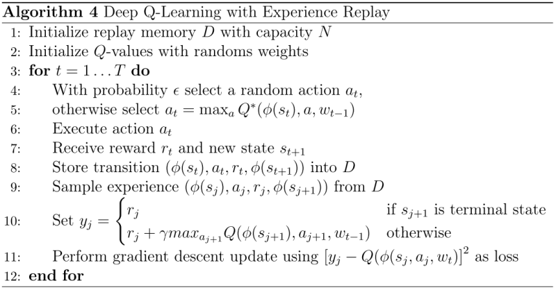
We now piece everything we have discussed so far into the Deep Q-Learning Algorithm (Mnih et al., 2013), given in Algorithm 4:

Notice that when we select an action using , we use the previous weights instead of the current weights .

I will now clarify the algorithm concerning the weights . Remember that in the loss function, to calculate the current prediction , we used the previous weights . What happens if ? We will use random weights. In implementation, this simply means we keep track of 2 weights: one of a past time step, and one of the current time step. Note that we would not necessarily need to use the weights immediately before . As long as it belongs to a past time step it will work (, where is a fixed constant).

Afterword

I took some material from Tambet Matiisen’s great series on Deep Q-Learning (Demystifying Deep Reinforcement Learning, Deep Reinforcement Learning with Neon), and also referred to his Simple DQN implementation. There is also some parts that I referenced from Freitas’s lectures on Deep Reinforcement Learning (part of their machine learning course).

References

• Bellemare, M. G., Naddaf, Y., Veness, J., & Bowling, M. (2013, 06). The arcade learning environment: An evaluation platform for general agents. Journal of Artificial Intelligence Research, 47, 253–279.
• de Freitas, N. (2014). Machine learning: 2014-2015. University of Oxford.
• Lin, L.-J. (1993). Reinforcement learning for robots using neural networks (Tech. Rep.). DTIC Document.
• Mnih, V., Kavukcuoglu, K., Silver, D., Graves, A., Antonoglou, I., Wierstra, D., & Riedmiller, M. (2013). Playing atari with deep reinforcement learning. arXiv preprint arXiv:1312.5602.